Leaks- An Investigation Into Inverse Problems
Carrie Nugent
12/03/07

Introduction

The process of leaking occurs frequently in nature, and is seen such diverse settings as the eruption of Enceledus’ geysers, the distribution of smoke emerging from the Centralia coal mine fires, and the leaking of air from an iron lung respiratory device. This simple investigation aims to determine the efficiency at which a detector can pinpoint the location of a leak.

This project is part of a collaboration with Sailor and Gretel Greene of the University of Texas at Austin’s ACTLab. Their contribution can be found on the website http://actlab.us/~sailor/three.html.

Model

We consider a two dimensional leak model, where regions of different pressures are separated by a thin membrane. Along this membrane are ten possible leak
sites. Synthetic data is generated by assigning the leak sites values of “off” (0) or “on” (1). This is accomplished by adjusting the m vector (See Figure 1). Using linear, steady-state diffusion (see G matrix, Table 1), a d vector is generated (where Gm=d). This d vector is analogous to a nine-node pressure detector located away from and between the leak points (see Figure 2).

Using least squares fitting and Tikhonov regularization, new m and d vectors are generated and compared to the originals. Although the problem is linear, it was found that nonsingular values introduced complexity into fitting. As this problem is roughly approximating a leak occurring along a seam of an iron lung, a few physical constraints can be placed on the resulting derived m vectors. The m values should not be negative, nor should they exceed a value of 1 (maximum allowed value).

Results

Several initial m vectors were tried, but for simplicity this paper will reference only two cases. The first, or localized case, is that of m=[0;0;0;0;0;0;1;1;1;0], where only the 7th, 8th, and 9th locations are leaking. The second, more challenging case to fit is that of an alternating m vector, where m=[0;1;0;1;0;1;0;1;0;1].

Synthetic d vectors were generated for the localized leak case, and new m vectors were solved for using a least squares fit. The singular values of the G matrix limited the effectiveness of these fits (Figure 2). Tikhonov regularization was used to set a lower limit on possible G values, and an alpha value was picked to minimize the residuals while still producing a physical answer.  Several different values of alpha were computed, and the curves corresponding to these different alpha values can be seen in Figure 4. Figure 4 should be compared with Figure 5, which displays the d vectors corresponding error bars (residual values). Note that the worst fit in Figure 4 corresponds with extreme residuals in Figure 5. However, all d vectors are within their error bars of the original d vector.

A comparison between the least squares fit and the Tikhonov fit can be seen in Figure 2.  Although the least squares fit was able to capture the basic character of the leak arrangement, it was not highly accurate. The Tikhonov fit looks much better in comparison, however it is worth noting that even this fit has significant deviations from the actual m vector. The Tikhonov regularization fit for this localized leak case is notable for being the most unique studied in this paper—a wide variety of alpha values all produce very similar m vectors. However, these m values are not the same as the original m value.

This process was repeated for the alternating leak case (Figure 6). Note that in this case, the pressures are equal at each of the detector points, and the fit must rely the edge conditions to determine the positions of the leaks. The least squares fit, while capturing the alternating nature of the leaks, did not pinpoint any of their locations. On the whole, the least squares fit was wildly inaccurate, and cannot be trusted. The Tikhonov regularization captured the symmetry of the leaks while failing to predict the relative magnitudes of the leaks. Once again, the Tikhonov fit only looks good while standing next to its neighbor, the least squares fit. However, since the Tikhonov fit can capture the basic nature of this challenging case, it is reasonable to assume that this method could accurately reproduce the character of any combination of leaking/ not leaking sites, though not necessarily the magnitude.

Figure 7 displays the d vectors for this case. Although the original d vector falls within the error bars for the least squares and Tikhonov regularization fits, the m vectors are highly non-unique.

Random errors with a standard distribution of 0.01 representing noise were then introduced into the localized case such that d=Gm+h, where h is the noise. This level of noise would be present in any physical system, and could be seen as accounting for instrument inaccuracies or the presence of very slight, brief motions of air not related to the leak. Both of these examples would produce noise that could reasonably be assumed to be random, with a normal distribution. When this was incorporated into the calculations, the resulting m vectors showed that even this very small amount of noise was enough to entirely sabotage both fits (Figure 8). When even this small amount of noise is incorporated, the Tikhonov fit becomes unreliable and the fitted model is not consistent with the data. As seen in Figure 9, the calculated d vector from this fit does not include the original d vector within its error bars.  The addition of this small amount of noise results in a problem too complex for Tikhonov regularization. A more advanced solution that took into account assumptions based on the noise and the nature of the leaks (positive, maximum of 1) could  more effectively tackle this problem.

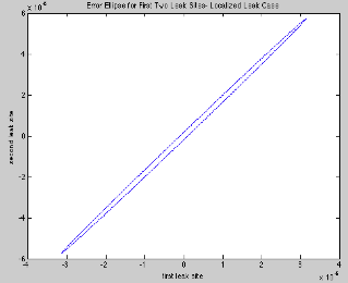
It is worth noting that in only one case did the model parameters approach uniqueness (see above). In all noiseless cases, however, the model parameters produced data that fit the original d vector within their error bars. Several modifications to the model could be made to ensure good fit, such as a higher detector/leak site ratio, detectors closer to leaks, or a higher pressure difference across the membrane. However, as detailed in the conclusion, these modifications would result a less realistic iron-lung model. To further investigate the difficulty of fitting, a 95% confidence ellipse was created for the first and second leak sites (Figure 10).  The ellipse is highly eccentric, illustrating the difficulty of the fit—finding the minimum in this parameter space requires small step sizes.

Conclusions

Using Tikhonov regularization to reduce the impact of the singular values, the main characteristics of the original m value can be reproduced. Deviations between the derived and original m vectors in the noiseless case are only due to the fact that this is an underdetermined problem.
 The addition of a very small amount of noise results in very poor fits, and the derived m values are wildly different from the original.  For this case, the model is not consistent with the data.

Physically, this model illustrates the difficulty of pinpointing leaks from a distance. In this model, the detector array was ten units away from the leaks, where the leak sites were one unit apart. The spacing between rivets (and therefore leak site spacing) on an actual iron lung is roughly two inches, indicating that a perfect detector at or less than twenty inches away would be able to pinpoint a leak. However, since noiseless real world detectors (and noiseless environments) are fictional, we can infer that a real world detector would need to be significantly closer to the iron lung to function properly.
Additionally, this model assumed that the pressure on one side of the membrane was double that of the pressure on the other side. Actual pressure differences used in an iron lung are less drastic- at maximum pressure, the interior has a roughly 1.45% increase in pressure (a very small amount!) [1]. Since the pressure drop-off is linear with distance, we can adjust our previous distance of 20 inches to account for this reduced pressure difference. Solving the simple ratio:
2 /0.0145 = 20 inches/ x inches gives a new maximum distance (without noise) of 0.145 inches for the detector. Clearly, a detector array as modeled in this paper is not an effective method for locating leaks on an iron lung. One would be far better off applying liquid over the leak points and looking for bubbles.

Reference

[1] Baisch, F. J., R. Gerzer, Breathing Assistance by the Iron Lung Increases Sympathetic Tone and Modifies Fluid Excretion,      IAF abstracts, 34th COSPAR Scientific Assembly, The Second World Space Congress, (2002), Houston, TX
            *Authors noted a pressure difference of 15 cm H2O, which I converted to approximately 0.01449 atm.

Tables and Figures

Table 1: G matrix.
The G matrix was generated assuming simple, steady state diffusion.

Figure 1: Model
Two regions of different pressure (light and dark purple) are separated by a membrane (black) with 10 possible leak sites (black rectangles). These sites can be set to leak or not leak—here, sites seven, eight, and nine are leaking. An array of nine detectors is situated above the leaks.  Note that the detector array is aligned such that the detectors are equidistant to the two nearest leak sites. The spacing between the leak sites is uniform and equal one tenth of the spacing between the detector array and the leaks. (Figure not to scale)

Figure 2: Localized leak arrangement. Leak sites seven, eight, and nine are leaking (corresponds with Figure 1), the remainder are off. Here the detected pressure at nodes 1-9 decreases with distance. For the following simulations, the detector is held at a fixed distance of 5, as seen on this plot.

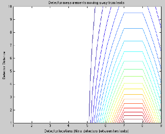
Figure 3. Least Squares Fit and Tikhonov Regularization for localized leak arrangement. Although the Tikhonov fit does more closely reproduce the original m matrix, note that it is by no means exact.

Figure 4- Tikhonov fit with a range of values for alpha=10^(alpha exponent). Compare with residuals of these fits shown in Figure 5.

Figure 5: Data (d) vectors and error bars (residuals) from Tikhonov fit for a range of values alpha=10^(alpha magnitude). Note that actual data falls within all error bars.

Figure 6. Least squares fit and Tikhonov regularization for alternating leak case. The least squares fit, while capturing the alternating nature of the leaks, did not pinpoint any of their locations. The Tikhonov regularization captured the symmetry of the leaks while failing to predict the relative magnitudes of the leaks.

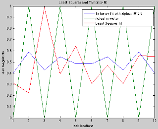
Figure 7: Data vectors with residuals for least-squares fit and fit using Tikhonov regularization. Again, actual data falls within all error bars.

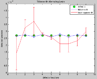
Figure 8: Least squares fitting and Tikhonov regularization with the addition of noise, Although the noise has a standard deviation of only 0.01, it is enough to befuddle both fitting algorithms. Both predict unphysical positive values significantly over 1 as well as negative values.

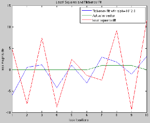
Figure 9: Generated data with noise using Tikhonov fit. Green circles are original data vector d for comparison. Note that one third of the actual values for d are outside the error bars (residuals).

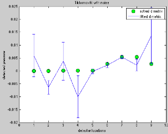
Figure 10: 95% Confidence Ellipse—Leak locations 1 and 2 (Tikhonov Fit, localized leak case, no noise). Note the long, narrow shape of this ellipse indicates a difficult parameter space to fit.

Word Document
PowerPoint Presentation

(C) 2007 Carolyn Nugent